Graphing basics

This longform guide covers what's achievable with Charts, how to use them with varying types of data, visual customisation, and points towards some advanced tricks!

Electric UI bundles our own graphing implementation designed specifically for high-performance realtime use. It's designed specifically for high performance, leveraging GPU acceleration and carefully tuned data handling backends to maximise performance and/or battery life on portable devices.

Performance scales nearly linearly if you try to draw one very high-speed variable, a dozen lines on one chart, or a dozen different variables on different charts[^1].

In our tests with mid-range compute resources (Intel 6-series iGPU) , we've demonstrated between 1-3 million points on screen with realtime datarates exceeding 50k points added per second. This is while reaching render targets above 120fps.

Getting Started

First, import the charting components we'll need and create a DataSource with the message identifier we want to chart.

import { 
  ChartContainer,
  LineChart,
  RealTimeDomain,
  VerticalAxis,
  TimeAxis
} from '@electricui/components-desktop-charts'
import { useMessageDataSource } from '@electricui/core-timeseries'

The datasource is responsible for filtering messages arriving from hardware, and then references those values against a timestamp in a format optimised for charting.

The actual datasource used here is a MessageDataSource and should be used through the useMessageDataSource React hook.

export const OverviewPage = () => {
  const sensorDataSource = useMessageDataSource('sensor')
  return (
    <React.Fragment>
      Chart will go here
    </React.Fragment>
  )
}

With the inbound data managed by a DataSource, we'll need to create something to display it.

Electric UI's charts are designed around a composability model - a ChartContainer provides the GPU accelerated (WebGL) context and accepts child components responsible for specific sections of the chart's functionality.

<ChartContainer>
  // Flat list of child functions will go here
</ChartContainer>

The container needs to be provided with a time reference, and how to control the window of data being displayed - RealTimeDomain is the most used, but other domain providers exist for specific use-cases.

<ChartContainer>
  <RealTimeDomain window={10_000} yMin={0} yMaxSoft={100}/>
</ChartContainer>

Adding axis lines, annotations and labels is as easy as adding the TimeAxis and VerticalAxis components to the ChartContainer.

<ChartContainer>
  <RealTimeDomain window={10_000} yMin={0} yMaxSoft={100}/>
  <TimeAxis />
  <VerticalAxis />
</ChartContainer>

The next sections will show you how to use these simple ideas to build different types of charts!

Realtime Charts

Data is drawn on the left of the chart as it arrives, and moves left as it 'ages'. The window is usually a fixed time period.

These charts are what most use-cases would expect to use for continuous real-time use.

With a datasource providing our timeseries data, use a LineChart to plot the data, with a RealTimeDomain to tell the chart to display a 10 second (10,000 ms) window.

<ChartContainer>
  <LineChart dataSource={sensorDS} />
  <RealTimeDomain window={10_000} />
  <TimeAxis />
  <VerticalAxis />
</ChartContainer>

Triggered Charts

Triggered charts draw a single window of data at once, without streaming/scrolling behaviour. When re-triggered, it will draw an entire window of data prior to the trigger point.

Best used when users need to evaluate the shape of the curve for longer periods of time, or when data is arriving at high rates while being viewed with a short duration window.

To trigger a redraw when a hardware sync message arrives, create a second datasource to act as the trigger. Instead of a RealTimeDomain, use a TriggerDomain and provide the new trigger source.

The TriggerDomain needs an accessor to select the time

import { TriggerDomain } from '@electricui/components-desktop-charts'

<ChartContainer>
  <LineChart dataSource={sensorDS} />
  <TriggerDomain
    dataSource={triggerDS}
    accessor={(event, time) => time}
    window={10_000}
  />
  <TimeAxis />
  <VerticalAxis />
</ChartContainer>

In situations where the trigger is a threshold on our signal of interest, we can write a custom DataSource which only emits events when our condition is met.

The logicalcomparison is oscilloscope behaviour, which can start drawing when a trigger condition is met. This behaviour is also well suited for drawing impulse-response charts when tuning a PID controller, or monitoring the behaviour of a system after a change in operating mode.

import { useDataTransformer } from '@electricui/timeseries-react'
import { filter } from '@electricui/dataflow'
 
let triggerMax: number = 90
 
const maxTriggerDS = useDataTransformer(() => 
  filter(sensorDS, (data, time) => data > triggerMax)
)

2D Charts

When working with sensor data which is best expressed with respect to another variable rather than time, a 2D plot (often called a XY plot) might be a better option.

These charts are useful when visualising GPS position trails, accelerometer XY readings aka G-Force indicator, or representing test-bench data.

Refer to the TimeSlicedLineChart component docs if you need a basic reference implementation.

Charting arrays & structures

Different datasources

Display many different data sources with the same ChartContainer by adding additional LineChart children.

const ambientTempDataSource = useMessageDataSource('ambient_c')
const cathodeTempDataSource = useMessageDataSource('cathode_c')

<ChartContainer>
  <LineChart dataSource={ambientTempDataSource} />
  <LineChart dataSource={cathodeTempDataSource} />
  <RealTimeDomain window={10_000} />
  <TimeAxis />
  <VerticalAxis />
</ChartContainer>

Array data

Charts follow the standard accessor syntax for accessing array elements. This allows you to directly access the array index of interest.

<LineChart
  dataSource={sensorArrayDS}
  accessor={state => state[0]}
/>
<LineChart
  dataSource={sensorArrayDS}
  accessor={state => state[1]}
/>

To plot an unknown number of values in an array, we can write a simple inline function to create as many LineChart children as needed.

To display all of the (unknown number) sensors, we need to know how many sensors we need to add, so we use the useHardwareState() hook to get the sensor state, then use .length to get the number of array items.

export const SensorDetails = () => {
  const numProbes: number | null = useHardwareState(
    state => (state.sensors || []).length,
  )
 
  return (
    <ChartContainer>
      {Array.from(new Array(numProbes)).map((_, index) => (
        <LineChart
          dataSource={sensorArrayDS}
          accessor={state => state[index]}
        />
      ))}
      
      // Domains, axis, etc...
    </ChartContainer>
  )
}

Structured data

Charting a member of a custom data type is almost the same as using array elements. The accessor specifies the target member of the custom type.

For this example, the temp message has three members containing different temperature readings.

const temperatureDataSource = useMessageDataSource('temp')
               
const temperatureDataSource: MessageDataSource<{
    furnace: number;
    exhaust: number;
    ambient: number;
}, "temp">

Using them in charts is just a matter of writing the accessor function:

<LineChart
  dataSource={temperatureDS}
  accessor={state => state.furnace}
/>
<LineChart
  dataSource={temperatureDS}
  accessor={state => state.ambient}
/>

Visual Customisation

Charts have been designed with customisation in mind. Line colour, thickness, dashed lines, axis ticks and formatting and more.

Annotations provide horizontal or vertical lines to callout key values, with optional rich content drawn anywhere on the chart.

Axis Labels

Either or both axis can be labelled to provide context to the data. Most charts will have a VerticalAxis and either TimeAxis or HorizontalAxis.

ChartAxis documentation describes formatting the axis tick values and grid density.

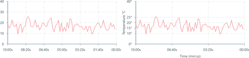
<ChartContainer>
  <TimeAxis label="Time (seconds)" />
  <VerticalAxis
    label="Temperature °C"
    tickValues={[0, 10, 15, 20, 25, 40]}
    tickFormat={(tick: number) => `${tick}°`}
  />
</ChartContainer>

Size and Color

LineChart accepts a HEX value or color alias string with color (docs).

Control the width of the line in 'pixels' with lineWidth (docs).

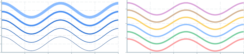
<LineChart dataSource={sensorDS} color="#0066CC" lineWidth={4} />
 
<LineChart dataSource={sensorDS} color={Colors.RED4} lineWidth={6} />

If specifying colours manually, be aware of contrast issues when using the same colours in light mode and dark mode.

To specify a colour for each mode, conditionally swap colour using the useDarkMode() hook as the driver.

import { useDarkMode } from '@electricui/components-desktop';

export const OverviewPage = () => {
  const darkMode = useDarkMode()
 
  return (
    <React.Fragment>
    <ChartContainer>
      <LineChart
        dataSource={sensorDS}
        color={darkMode ? '#559a75' : '#81ebb2'}
      />
      <TimeAxis />
      <VerticalAxis />
    </ChartContainer>
  </React.Fragment>
  )
}

Annotations

Annotations are used to provide callouts for a key feature(s) on the Chart. This could be to indicate a setpoint for an alarm, a threshold for a sensor, or to make the maximum of the curve more easily readable.

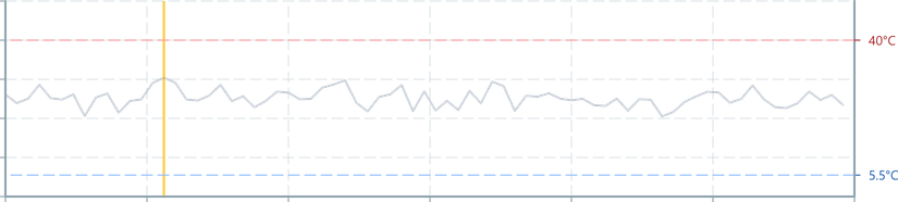
In this example, we'll display threshold lines with a label on the right-hand side of the chart using YAxisAnnotation, and display the maximum value with a VerticalLineAnnotation.

import { useDataTransformer } from '@electricui/timeseries-react'
import { max } from '@electricui/dataflow'
 
export const ChartPage = () => {
  // Create dataSources to drive the annotation values
  // This message is a custom type with 'low' and 'high' values
  const thresholdDS = useMessageDataSource('temp_limits')
  
  // DataTransformer to find the max value in our window
  const maxValueDS = useDataTransformer(() => max(sensorDS))
 
  return (
    <React.Fragment>
      <ChartContainer>
        // ...
 
        <YAxisAnnotation
          dataSource={thresholdDS}
          accessor={state => state.low}
          color={Colors.BLUE3}
        />
        <YAxisAnnotation
          dataSource={thresholdDS}
          accessor={event => event.high}
          color={Colors.RED5}
        />
 
        <VerticalLineAnnotation
          dataSource={maxValueDS}
          accessor={(data, time) => time}
          color={Colors.GOLD4}
        />
      </ChartContainer>
    </React.Fragment>
  )
}

Controls for visual properties such as colour, grid-line style and rendering behaviour are detailed in the annotations API reference.

Ordering

The render-order of a ChartContainer is from the top to the bottom. If you're trying to draw a specific chart or annotation above another, add it later in the component.

<ChartContainer>
  <LineChart dataSource={dataSource} color={Colors.RED5}/>
  <ScatterPlot
    dataSource={dataSource}
    accessor={(data, time) => ({ x: time, y: data })}
    color={Colors.BLACK}
  />
  {/* Axis, domain, etc */}
</ChartContainer>

<ChartContainer>
  <ScatterPlot
    dataSource={dataSource}
    accessor={(data, time) => ({ x: time, y: data })}
    color={Colors.BLACK}
  />
  <LineChart dataSource={dataSource} color={Colors.RED5} />
  {/* Axis, domain, etc */}
</ChartContainer>

Advanced Features

The Charting engine can do a lot more than just plot lines as data comes in.

A lot of the power behind detailed and useful charts is the ability to process data on the UI computer to provide additional context to a signal. This is done at the DataSource level with DataTransformers.

Additionally, there are graphics tricks which can heavily stylise charts during the render step. This is possible because Charts are backed by WebGL, allowing shaders to be applied to geometry and the scene.

Data Transformers

UI-side processing of inbound data helps provide things like realtime filters, averaging, or custom mathematical transforms. This is detailed in the Datasources guide.

For a more advanced example, we provide a copy-paste example for realtime Fast Fourier Transforms (FFT).

[^1]: A maximum of 16 ChartContainers can be drawn on one screen by default - contact us if you need to raise this limit.